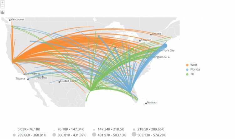
Improving supply chain logistics with geographic proximity matching
… The post Improving supply chain logistics with geographic proximity matching first appeared on Blog.

For a third-party logistics company like RWI Logistics, geographic data can be a crucial tool for solving problems and creating solutions for our customers. We often need to look up whether we’ve managed any truckloads into or out of a list of geographic areas. But it can be challenging to quickly match locations if they have a different city, state, and postal code from one another.
For example, if we wanted to know how many loads we’ve delivered in the vicinity of Fort Thomas, Kentucky, the simplest solution would be to search for past transactions with “City” = ‘Fort Thomas’ and “State” = ‘KY’. However, this method would not return transactions for Cincinnati, Ohio, despite the fact that Cincinnati is only 5 miles from Fort Thomas, because the city and state don’t match our specific search criteria.
Domo has enabled us to implement an efficient and repeatable solution to this problem. Our method uses Redshift dataflows and the Domo Dimensions Connector to match locations within a specified mileage radius, rather than relying on drawn boundaries like state lines.
There are three datasets required for this process:
- Location list – A postal code list for desired locations, such as potential new customer delivery locations.
- Transaction history – A list of past locations to search, containing postal codes.
- Domo Dimensions Connector “cityzip.csv” report – We will use this dataset to look up the latitude and longitude of each location.
Step 1 – Aggregate latitude/longitude table
Some postal codes appear in the Domo Dimensions dataset multiple times, so we must use a table transform in Redshift to aggregate this table so there is one row per postal code to avoid duplicating rows when we join to the other tables.
select
  "Postal",
  avg("Latitude") as "Lat",
  avg("Longitude") as "Long"
from "city_zip"
group by "Postal"
Step 2 – Transform locations into points on the globe
We first need to find the coordinates of the postal codes in the location list and transaction history by joining both datasets to the aggregated latitude/longitude table by postal code. The st_point() function transforms the latitude and longitude of each postal code into a point on the globe. Note that running SQL previews will not display any data when these points are included in the query.
select | select |
Step 3 – Join datasets
Now that the location list and transaction history both contain points, we can use the st_DistanceSphere() function to calculate the distance (meters) between points. We use this distance as the criteria for the join between the two tables. In this example, we match locations and transactions that are within 100 miles of each other.
select
a."postal",
a."location name",
b."transaction #",
b."location name" as "transaction location name"
from "location_coord" as a
left join "history_coord" as b
on st_distancesphere(a."coord",b."coord") <= 1609.34*100
Step 4 – Visualize results
Using the above transform as the output of the Redshift dataflow, we then create a summary card that displays the count of historical transactions by location name. We can also gather more context by drilling to the transaction detail.
Since implementing this process, RWI Logistics has improved the efficiency and consistency of location-matching tasks. Domo has given us the ability to quickly analyze location data for various use cases and share insights across the organization.
The post Improving supply chain logistics with geographic proximity matching first appeared on Blog.


